The Riemann Hypothesis, Part 1, Explained Simply
Levent Alpöge announced a Claude-assisted proof of the Riemann hypothesis on November 20. Lean and Mathlib reviewers reported that the formal proof passed independent checks. Clay still lists the problem as unsolved as of November 21. I wanted to write about it and look into what had actually been proved. It’s a big, emotional moment for a lot of mathematicians. People have been trying to prove this since 1859.
Why count primes in the first place? In 1859, Riemann was trying to understand how often primes show up as numbers get bigger. Gauss had already guessed a smooth estimate for the count. Riemann found a way to explain the bumps in the actual count using zeta. Today, knowing how dense primes are helps you work out how many candidates you might have to try when looking for a large prime, for example when generating an RSA key. Riemann’s 1859 paper · NIST’s prime-generation standard
We can already compute exact counts. If we could do it cheaply at huge scales, we could subtract two counts to see exactly how many primes are in a range, or find the millionth prime by looking for where the count first reaches a million. The Riemann hypothesis answers a different question. How far off can our estimate get as we count farther out? An algorithm for exact prime counts
Here’s the claim we’re working toward. Every nontrivial zero of the Riemann zeta function has real part ½. Okay, but why are we talking about a function when we want to count primes?
Primes go into zeta
Euler wrote zeta’s sum over whole numbers as a product with one factor per prime. For 12, the pieces come from 2 and 3, because .
The zeros tell us about the count
Riemann found that the inputs where zeta gives zero show up in terms that raise or lower a smooth estimate of the prime count. Where the zeros sit affects how large those corrections can get.
For example, the smooth formula estimates about 78,628 primes up to a million. The actual count is 78,498. That’s the kind of gap we’re trying to understand as we go farther out. The hypothesis ties a limit on that gap to the line through ½. We’ll come back to how that works. Riemann’s 1859 paper
Where Do Prime Numbers Appear?
Prime numbers are whole numbers greater than 1 divisible only by 1 and themselves. 2, 3, 5, 7, 11, 13, 17, 19… They are the building blocks of whole numbers. For example,
Every whole number greater than 1 has a unique prime factorization, apart from the order. But the primes themselves appear irregularly. Sometimes they are close together, like 11 and 13. Sometimes there is a much larger gap. One way to see their patterns is to arrange whole numbers in an outward square spiral, then highlight the primes. This is called an Ulam spiral. Diagonal patterns start appearing.
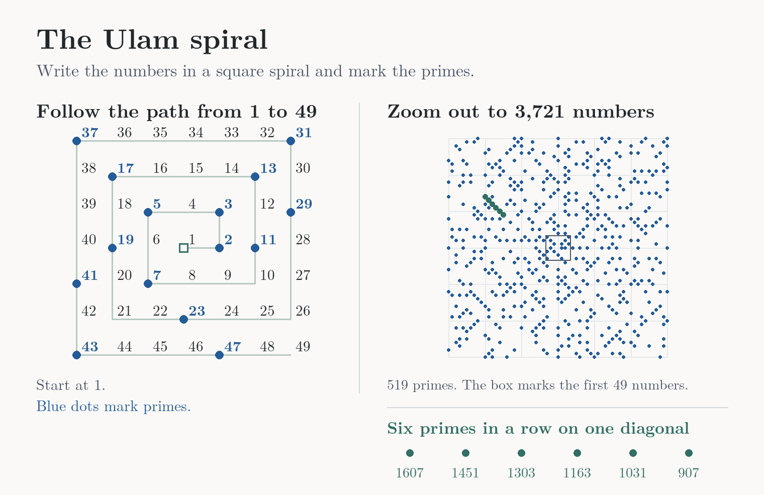
Same spiral, zoomed out. The six green dots are primes next to each other on a diagonal.
I am an atheist, but seeing that prime numbers form mysterious shapes and patterns is a religious experience for me, reaching the limits of human intuition. We chose the spiral arrangement, so the picture depends on how we display the numbers. Still, the concentrations of primes along some diagonals are interesting mathematical patterns. The Riemann hypothesis concerns another kind of regularity. How many primes appear as we move further along the number line?
Counting Primes
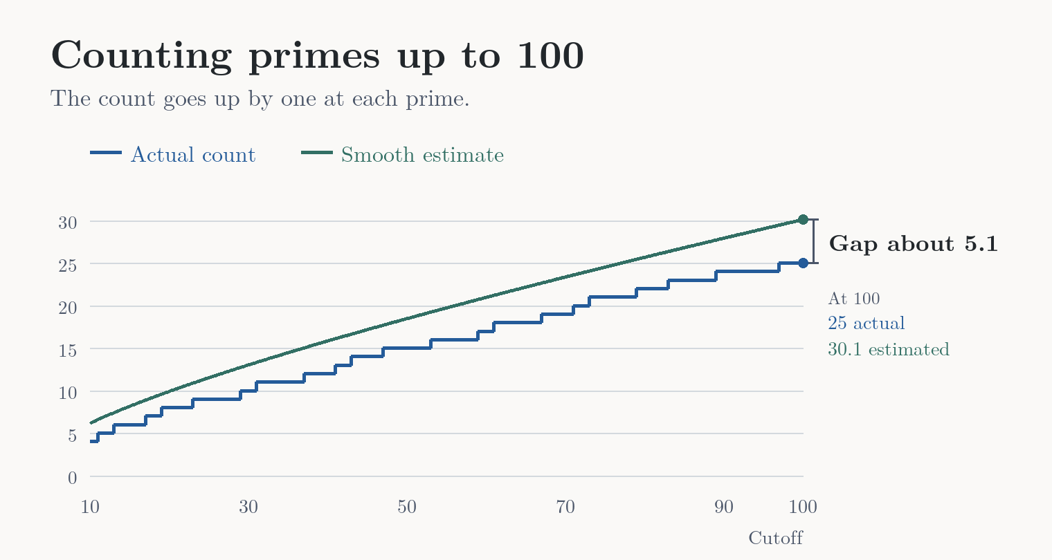
There are 25 primes up to 100. Draw the count as a staircase and each prime takes you one step up. The smooth curve gives an estimate of about 30 at the same cutoff. So it’s about five too high there. The Riemann hypothesis puts a limit on how far apart those two can get as we count farther out.
What The Zeta Function Does
The Riemann hypothesis says that every nontrivial zero of the zeta function has real part ½.
A function takes an input and gives you an output. Feed me chocolate, I turn happy. Zeta's recipe involves a lot more fractions.
Zeta takes a number we call s. Plot by going two units right and three up. The two is the real part, the three is the imaginary part, and s is the whole point. Writing 2 is shorthand for .
How Zeta Is Defined
The original definition of the zeta function is this infinite sum. It defines ζ(s) when Re(s) > 1, meaning the real part of the input is greater than 1.
Use the same s in every exponent. At , that gives 1 + ¼ + ⅑ + 1/16 + ⋯. The running total settles near 1.645. That’s what converges means. A function is defined at an input if it gives that input a value.
At and , the running total keeps growing. At + i it also fails to settle, though the terms now turn in different directions. The sum converges exactly when Re(s) > 1. That means strictly right of the vertical line through 1.
What Is Extended Zeta?
Extended zeta gives the same answers wherever the original sum converges. It also gives values on and to the left of the line through 1, with one exception. At the single point 1 + 0i, zeta has a pole and no finite value.
From here on, ζ means the full function.
What is ζ(s)?
- If Re(s) > 1
- If Re(s) ≤ 1 and s ≠ 1
Use the longer recipe here. It’s called Hasse’s formula, and the value it gives you is ζ(s).
- If s = 1 + 0i
- There’s a pole. Zeta has no finite value.
You can plug any complex number except 1 into Hasse’s formula. Try it on the right of the line and you get exactly the same answer as the original sum.
Where did those coefficients come from? The idea is to work with differences between neighboring powers. Subtract two neighbors, then subtract two neighboring differences. That second step gives the pattern 1, −2, 1. Keep going and you get the alternating binomial coefficients in the first line. The derivation shows that the weighted groups add up to the original zeta value once you divide by s − 1. Those groups also give a convergent series at inputs where the original sum fails. Hasse’s formula and its derivation, equation 11
The first line makes one group of terms, called Aₙ(s). The second adds those groups after dividing each by n + 1. The stacked n and k mean “n choose k.” Try . The original sum is 1 + 1 + 1 + ⋯. In Hasse’s formula the first two groups give 1 and −½, and the rest cancel. Divide by −1 and you get .
In the diagram, blue marks where the original sum works. Green marks where the extension adds values. Real part 1 is the whole vertical line. The input 1 means , a single point on that line. Start at 1 on the horizontal axis and go straight up or down. Your horizontal coordinate stays fixed. At , one step above the pole, extended zeta has a finite value.
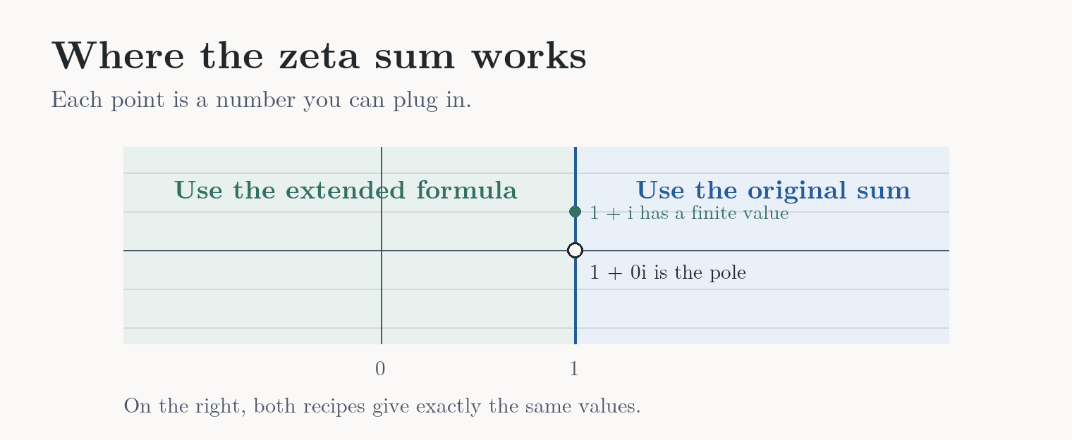
Each dot would be a number you can plug into zeta. The shading tells you which formula to use.
How Analytic Continuation Works
Why go farther? Riemann was looking for a way to count primes. The zeros that give corrections to the estimate live in the strip between real parts 0 and 1. The original sum can’t reach them.
How do you find a formula that does this? One way to see the idea is to flip the sign of every other term. At ½, the alternating terms cancel enough for the sum to settle. A factor in the denominator makes this formula match the original on the right. Derivation of the alternating formula
Why is there only one extension? Two analytic functions that match on an open patch have to keep matching throughout the connected region where both work. I love this. Those answers on the right pin down the answers farther left. MIT’s notes on the identity theorem
See the original and alternating formulas side by side
Original sum
Alternating formula
The domain diagram shows which inputs each formula covers. The stills below show what happens on the output side. Each curve traces the zeta outputs for a line of inputs. In the second still, more of each input line is available, so its output curve continues farther. The parts of the curves we already had stay where they were.

Outputs from the original sum. The numbers on these axes are coordinates of the output. For example, . The input has real part 2, and its output has real part about 0.8. The original sum can give an output to the left of 1 because the cutoff applies to the input.

Zeta outputs after analytic continuation. Extended zeta gives a value at and at inputs farther left, so the arc can keep going. The extra curves plot these new outputs. The short sum on screen is the starting recipe. 3Blue1Brown’s visual explanation
The colored still shows where the grid goes. To see one zero, follow just a short stretch of the input line through ½. Look at what happens to its output curve.
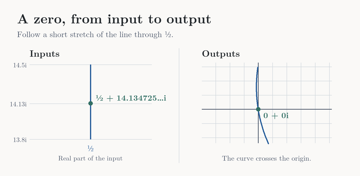
The green dot on the left is the input ½ + 14.134725…i. The green dot on the right is its output, 0 + 0i. The height matters. Plug in just ½ and you get about −1.460, so that particular point on the line is not a zero.
I love seeing this in motion. In 3Blue1Brown’s video on zeta and analytic continuation, you can follow a straight line of inputs as zeta turns it into a curve of outputs.
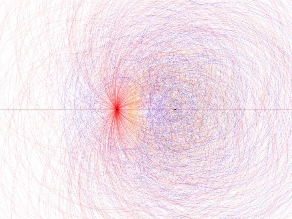
A Twitter user named Vivek shared this illustration. In a zeta plot like this, each curve traces the outputs as you move along a straight line of inputs. One reply called it a butthole. Vivek’s original post.
The Two Zeta Recipes
Both recipes take the whole complex number s as input. Re(s) is its horizontal coordinate.
- The original sum works when Re(s) > 1. For example, 2 + 3i works because its real part is 2. The 3 tells you the height of the input.
- Extended zeta works everywhere except at . At it gives exactly the original sum’s answer. At it gives an answer too, even though the original sum diverges there. The difference is which inputs have an answer. On their shared region, the answers are identical.
The two vertical lines have different jobs. The line through 1 marks the boundary of the original sum. The line through ½ is where the Riemann hypothesis says the nontrivial zeros lie. Analytic continuation lets us ask which inputs there give an output of zero.
As s approaches , the magnitude of ζ(s) grows without bound. At that exact input there’s no finite output. The hypothesis is about the inputs where the output actually equals zero.

I’m from Prague, where there’s a legend about a clay Golem that comes to life when a parchment is placed in its mouth. Get close to one particular value and a quiet-looking function turns into an uncontrollable creature.
What Is A Zero Of A Function?
Imagine a glass of wine is my input. I get tired and shut down. My output is zero. In that very scientific model of me, the glass of wine is a zero.
A zero of zeta is an input that lands at the origin of the output grid. That output is . Zero across, zero up. It’s where the two axes cross.
The Riemann hypothesis says that every nontrivial zero of zeta has real part ½. So the number ½ describes where those inputs sit on the grid. Their output is zero.
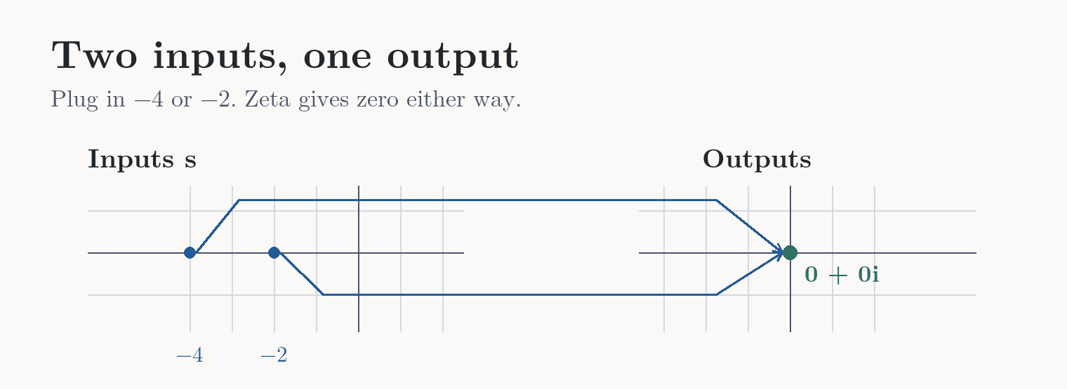
For example, −2 and −4 both land on that same dot. When we ask where the zeros sit, we go back to the input grid. That’s where the line through ½ lives.
A side note on “nontrivial.” The hypothesis says every nontrivial zero has real part ½. The obvious family, once you know where to look, is −2, −4, −6, and so on. Mathematicians already know exactly where those zeros are. The hypothesis is about the rest, in the strip between real parts 0 and 1. The two kinds of zeros
Why ½?
The real part is the horizontal coordinate. Saying all the nontrivial zeros have real part ½ means they all sit somewhere on the vertical line through ½. Here are three known examples.
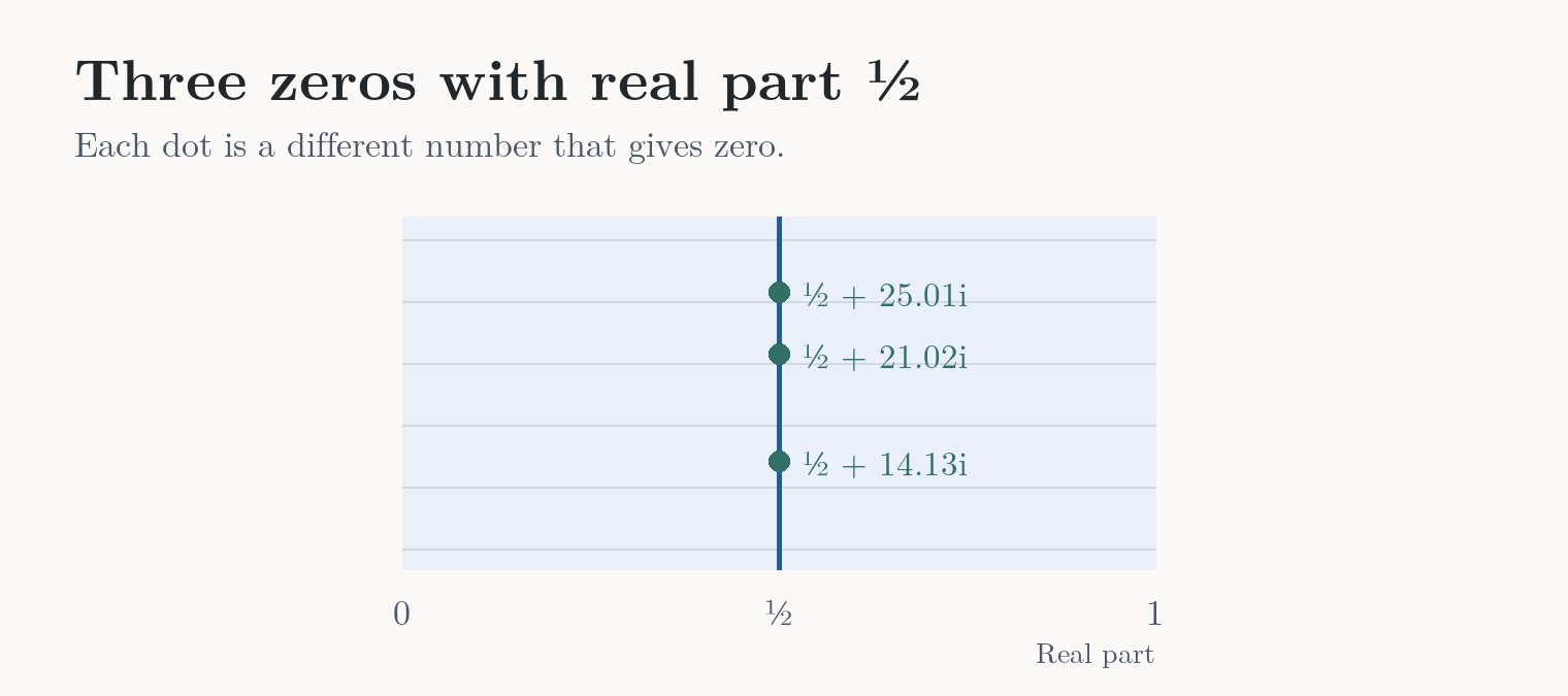
Inputs. Each dot gives the same output, zero.
We are used to symmetry around zero. On that number line, reflection sends 3 to −3. Zeta has a different rule. Riemann showed that his completed zeta function, called , has exactly the same zeros inside the strip and satisfies
For zeros, that symmetry, together with reflection across the real axis, pairs a horizontal coordinate with at the same height. The completed zeta symmetry
Think of 0.3 and 0.7. They add up to 1, so their midpoint is ½. Every reflected pair has this same midpoint. The only horizontal coordinate that stays put is the one that satisfies , which gives . That’s why the center is ½. Symmetry still allows off-line pairs. Ruling those out is what the hypothesis asks us to do.
Where the symmetry comes from
Riemann used an integral to express completed zeta, . Hasse’s series gives ζ directly. This formula gives ξ, which is ζ multiplied by factors that are finite and nonzero inside the strip. The two functions therefore have the same zeros there. The letter is a variable inside the integral, and is the same weight for both powers.
Replace with and the two powers of swap places. The factor in front stays the same too. So the whole expression has the same value. Riemann’s integral representation
The Hypothesis Recap
Every nontrivial zero of the Riemann zeta function has real part ½.
- Every.
- The proof has to cover all of them at once. One off the line would be enough to disprove it.
- Nontrivial zero.
- An input with output zero in the strip between real parts 0 and 1.
- Riemann zeta function.
- Start with 1 + 1/2s + 1/3s + ⋯ for Re(s) > 1, then use analytic continuation to reach the strip.
- Real part ½.
- Go to ½ on the horizontal axis and draw a vertical line.
How The Primes Get Into Zeta
Go back to the original sum. It has a term for every positive whole number. Euler showed that when Re(s) > 1, the same sum equals a product with one factor for each prime.
This is Euler’s product formula. The reason it works is that every whole number greater than 1 can be written as a product of primes in exactly one way, apart from order. For example, . The 2 factor supplies 1/4s, the 3 factor supplies 1/3s, and multiplying those gives the term 1/12s in the sum. Every number gets its one term this way. Euler’s product and its derivation
Counting Primes Up To A Million
Pick a number on the horizontal axis. That’s the cutoff, the number you count up to. At 70, the blue staircase is at 19 because there are 19 primes up to 70. The green curve gives the estimate for the same cutoff. The blue line takes a step whenever you pass a prime. The smooth curve, called Li(x), adds up the expected density of primes as you move along the number line. Near a large number, that density is roughly one prime per natural log of that number.
The formula for the smooth estimate
Li is short for logarithmic integral. Here we use the convention that starts at Li(2) ≈ 1.045 and adds the area under the reciprocal of the natural log.
At one million, we can get the exact answer by listing the primes, for example with a sieve. There are 78,498. Evaluate the smooth formula at the same cutoff and you get about 78,628. So Li is about 130 too high there. At another cutoff it could be too low.
The ordinary count at a million is about 130 below the estimate. The question Riemann was after is how big that gap can get as we count farther out. His route goes through a second count where the steps have different sizes. Riemann’s prime-counting formula
Counting With Weights
The ordinary count gives each prime a step of size 1. The weighted count gives a prime or prime power a step of size log of its base prime. The weight is a number you add when you reach that entry. For example, the natural log of 2 is about 0.69.
2 is prime
Ordinary step +1
Weighted step +0.69
4 is 2²
Ordinary step 0
Weighted step +0.69
6 is 2 × 3
Ordinary step 0
Weighted step 0
Four gets a weight because it’s made by repeating one prime, 2. Six mixes two different primes, so it has no step in either count. You can calculate the weighted count exactly by adding the prescribed weights. We’ll estimate that total separately.
| Number | Prime or factorization | Primes added | Weight added |
|---|---|---|---|
| 2 | Prime | 1 | log 2 |
| 3 | Prime | 1 | log 3 |
| 4 | 2² | 0 | log 2 |
| 5 | Prime | 1 | log 5 |
| 6 | 2 × 3 | 0 | 0 |
| 7 | Prime | 1 | log 7 |
| 8 | 2³ | 0 | log 2 |
| 9 | 3² | 0 | log 3 |
| 10 | 2 × 5 | 0 | 0 |
| 11 | Prime | 1 | log 11 |
At a cutoff of 11, the ordinary total is 5 primes. The weighted total is about 10.23, from adding the logs in the last column.
The weighted count has a simple starting estimate. Up to 125, start at 125. Near a large cutoff, primes show up roughly once per log of that number, and each prime adds roughly that same log as its weight. Those two effects balance, so the weighted total grows about as fast as the cutoff.
How The Zeros Give Corrections
Euler’s product is zeta written with one factor per prime. It agrees with the original sum when Re(s) > 1.
Working with this product gives a formula for the weighted count. It starts from the smooth estimate and adds terms that depend on the zeros. The chart below isolates one of those terms after pairing two zeros.
The pair comes from the zeta input grid. is above the real axis and is below it, at the same distance. Both are nontrivial zeros with real part ½. Mathematicians combine their contributions because the imaginary parts cancel and the result is a real adjustment you can add to the count.
What One Correction Looks Like
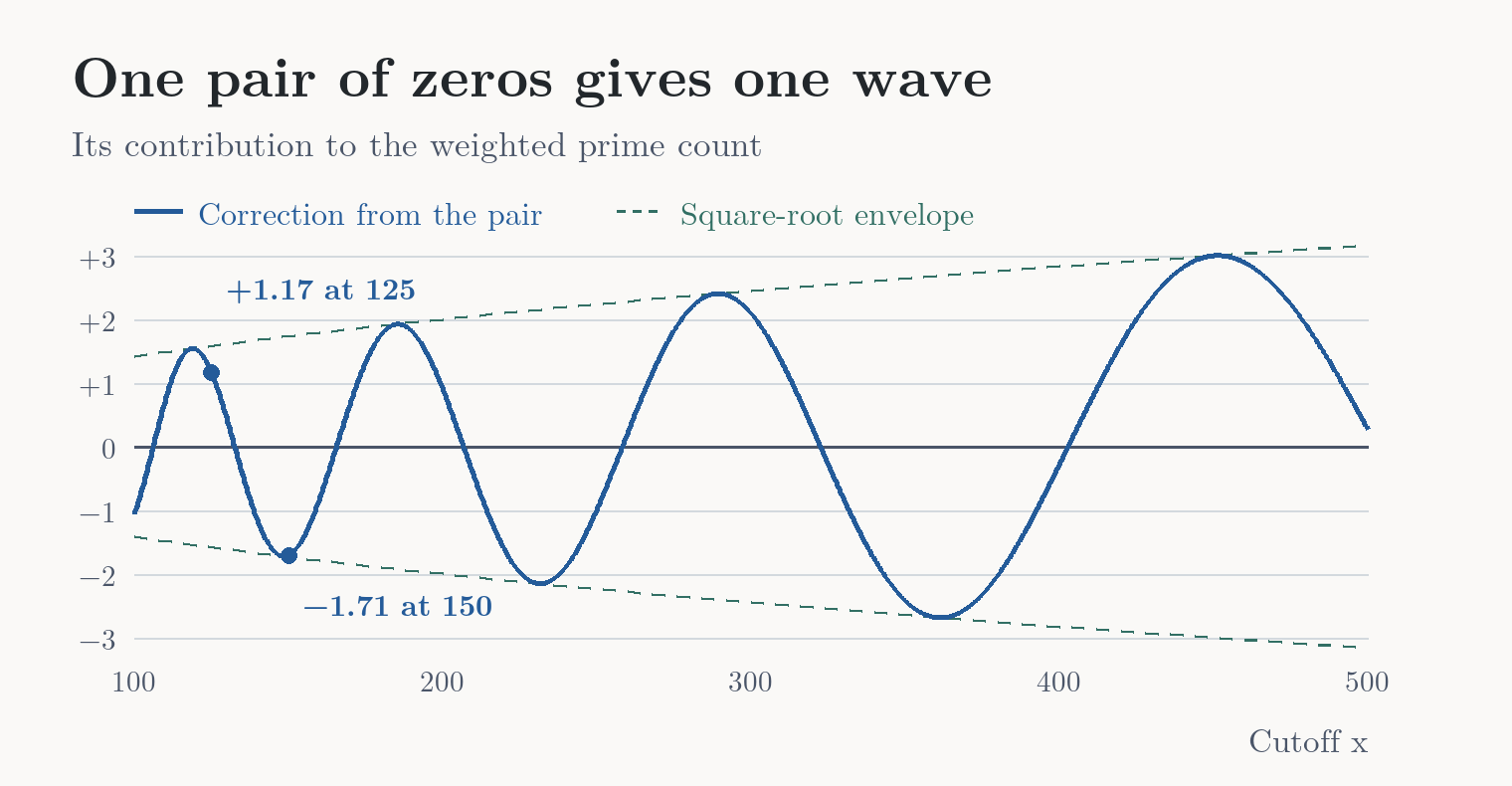
The horizontal axis is how far we count. The vertical axis is how much this pair adds to or subtracts from the weighted estimate. The dashed green lines bound this one blue wave.
At 125, this pair adds 1.17 to the starting estimate of 125. At 150, it subtracts 1.71 from the estimate of 150. Those are changes to the weighted estimate. The heights of the two zeros stay fixed at about +14.13 and −14.13 on the zeta input grid. The formula for the weighted count
The formulas behind the chart
The negative derivative of the logarithm of Euler’s product brings down the log weights. On the zeta side, that gives the quotient below. At a zero of zeta, its denominator goes to zero one power faster than its numerator, so the quotient has a pole there.
Recovering the weighted count from the quotient turns the pole at each nontrivial zero, written ρ, into the contribution below. Here x is the cutoff. Combine this with the term from the zero at the opposite height and the imaginary parts cancel. That pair gives the real wave in the chart.
Where The ½ Shows Up
The ½ belongs to the input that makes zeta zero. It shows up in this chart as an exponent. For that pair, the dashed green lines move away from zero in proportion to the cutoff raised to the power ½. That’s the square root. From 125 to 500, the cutoff quadruples and the maximum size of the wave doubles. The blue wave can still be anywhere between those dashed lines.
We already know the two zeros used in this chart sit on ½. The hypothesis says that every nontrivial zero does. That would give each pair a square-root limit on its own wave. A zero farther to the right would allow a faster-growing contribution. The formula connecting zeros and the weighted count
What The Hypothesis Says About The Counting Error
The blue wave is one piece of the weighted calculation. To translate the full weighted staircase back into an ordinary count, keep the steps at primes and change their sizes to 1. For example, the weighted step at 2 becomes a step of size 1. The weighted step at 4 disappears because 4 is a higher power of 2.
A bound is a limit on how far the estimate can be from the count. At a million we measured a gap of about 130. The hypothesis gives a general limit for large cutoffs after mathematicians control all the waves together and translate back to the ordinary count. That limit grows on the scale of the square root of the cutoff times its logarithm. The prime-counting error bound
The error bound in mathematical notation
The left side is the actual number of primes up to x. The O term says that, once x is large enough, the absolute gap stays below a fixed constant times the square root of x times log x.
In Part 2, I look at how the argument works, what the independent Lean checks established, and what to make of the competing claims.